Code
library(gt)
library(tidyverse)
library(patchwork)
library(bggjphd)
theme_set(theme_bggj())library(gt)
library(tidyverse)
library(patchwork)
library(bggjphd)
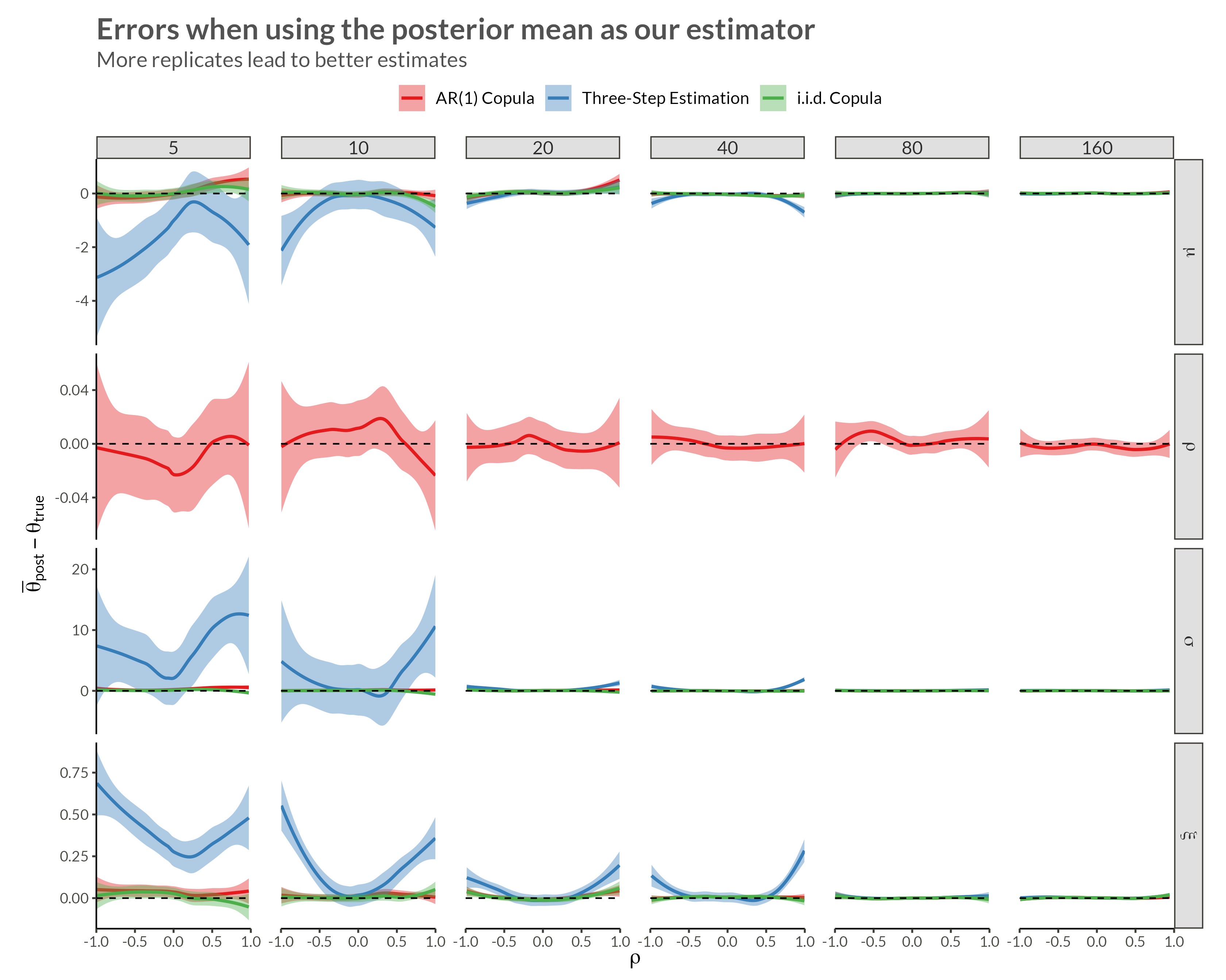
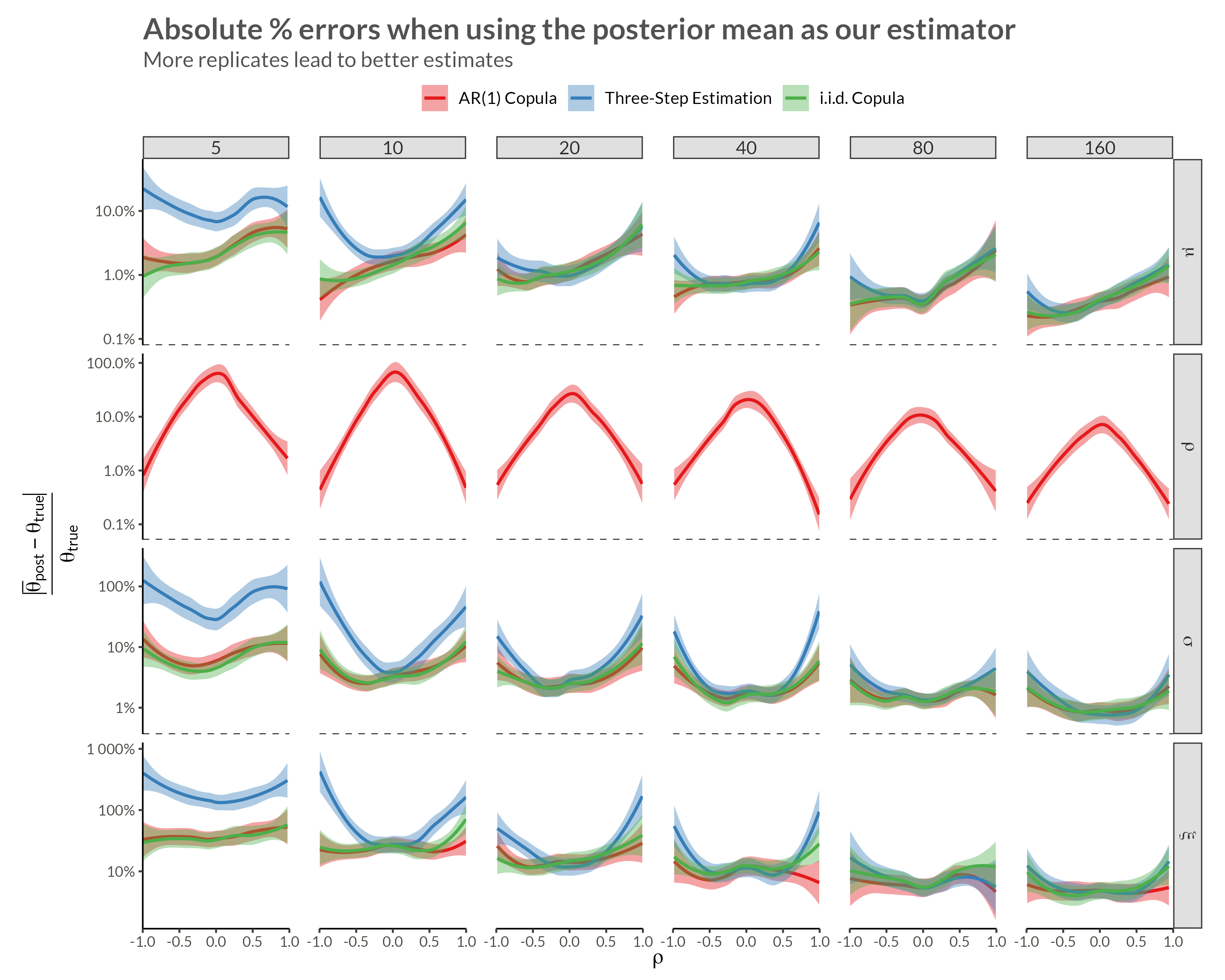
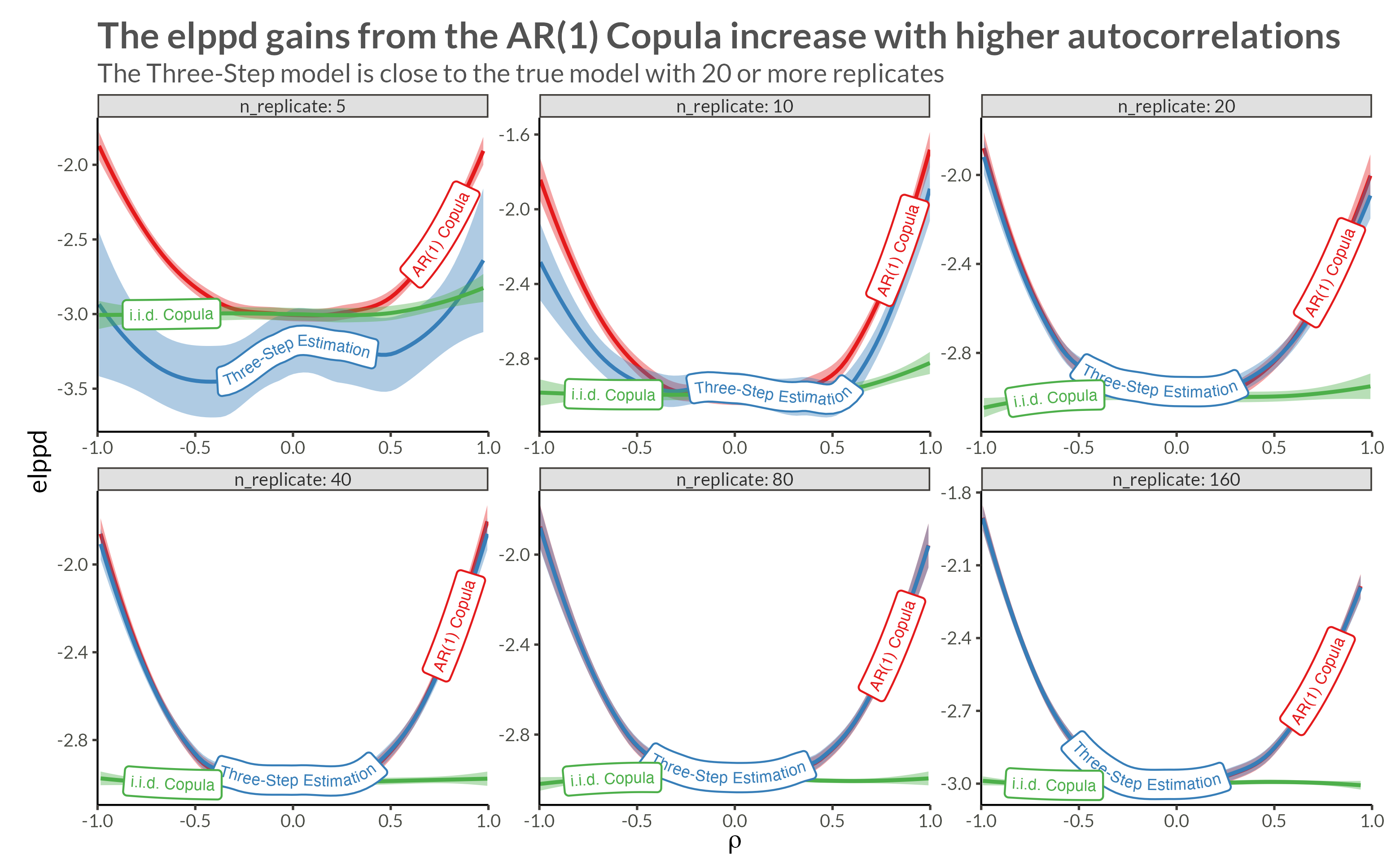
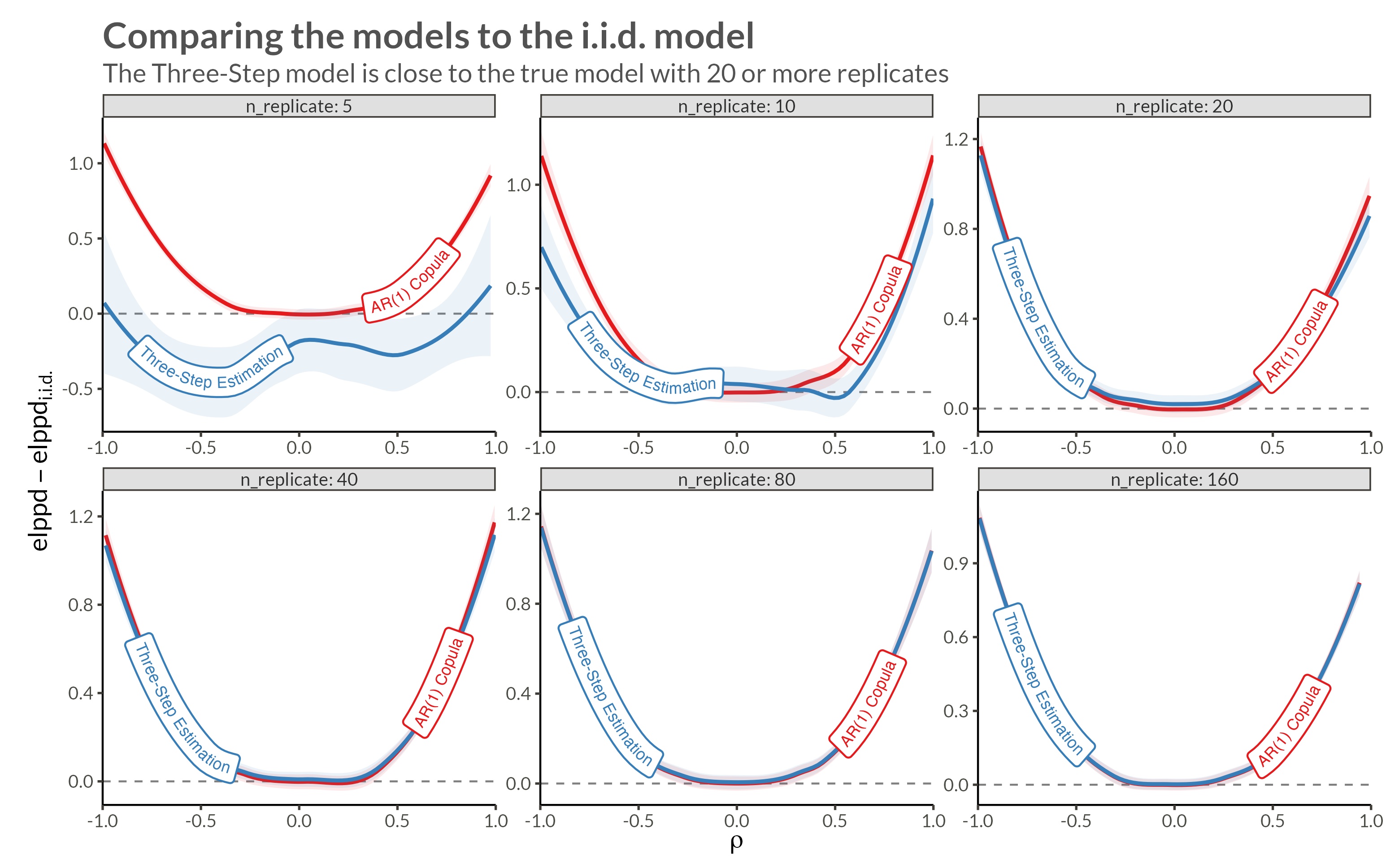
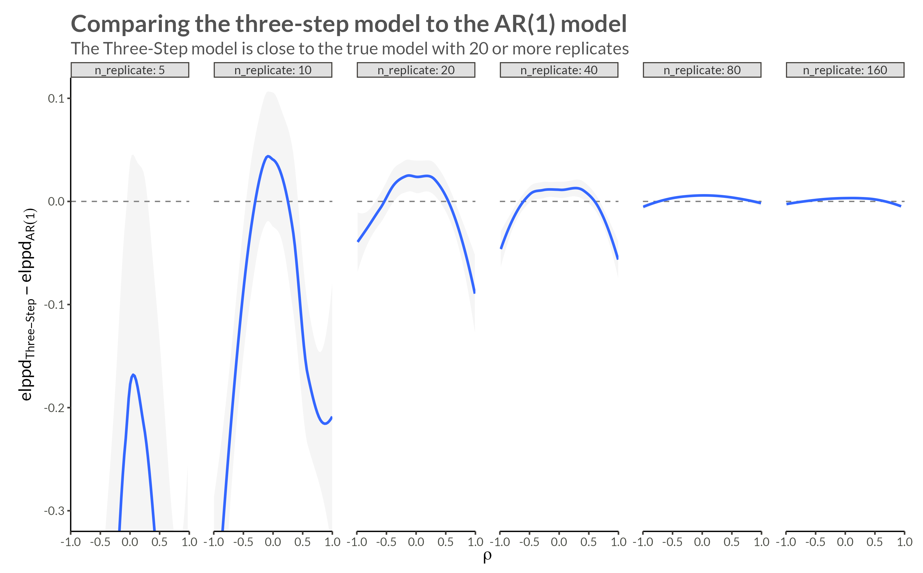
theme_set(theme_bggj())In a previous post, I wrote about applying the BYM2 model to spatially dependent Generalized Extreme Value (GEV) data and mentioned in passing that I was working on applying copulas as well. In this post I will outline and show results from a simulation study I’ve been running where I:
In the book Elements of Copula Modeling with R, Hofert et al. (2018) define a copula as
a multivariate distribution function with standard uniform univariate margins, that is, U(0, 1) margins.
So, a Copula is any multivariate distribution whose margins is U(0,1 ) distributed. A simple example is the independence copula
\[ \Pi(u) = \prod_{j=1}^{d}{u_j}, \quad \mathbf U \in [0, 1]^d. \]
The central theorem of copula theory is Sklar’s theorem (Sklar 1996) [the original paper is from 1959]. The theorem basically states that for any d-dimensional distribution function, \(H\), with univariate margins \(F_1, \dots, F_d\), there exists a d-dimensional copula \(C\) such that
\[ H(\mathbf x) = C(F_1(x_1), \dots, F_d(x_d)). \]
Alternatively, we can write
\[ C(\mathbf u) = H(F_1^{-1}(u_1), \dots, F_d^{-1}(u_d)) \]
The Gaussian family of copulas can be written
\[ C(\mathbf u | R) = \Phi_d\left(\Phi^{-1}(u_1), \dots, \Phi^{-1}(u_d) \vert R \right), \quad \mathbf u \in [0, 1]^d, \]
where R is a \(d\times d\) correlation matrix, \(\Phi_d\) is the CDF of a d-dimensional multivariate Gaussian with mean \(\mathbf 0\) and covariance matrix \(R\), and \(\Phi\) is the CDF of a standard Gaussian.
Its density is
\[ c(\mathbf u \vert R) = \frac{\phi_d\left(\Phi^{-1}(u_1), \dots, \Phi^{-1}(u_d) \vert R \right)}{ \prod_{j=1}^{d}{\phi\left( \Phi^{-1}(u_j) \right)}}, \quad \mathbf u \in [0, 1]^d, \]
where \(\phi_d\) is the density of the same multivariate Gaussian, and \(\phi\) is the density of a standard gaussian.
Given the \(d\times d\) correlation matrix, \(R\):
We can then make the margins \(u_1, \dots, u_d\) follow any distribution (f.ex. the GEV distribution) by applying its quantile function.
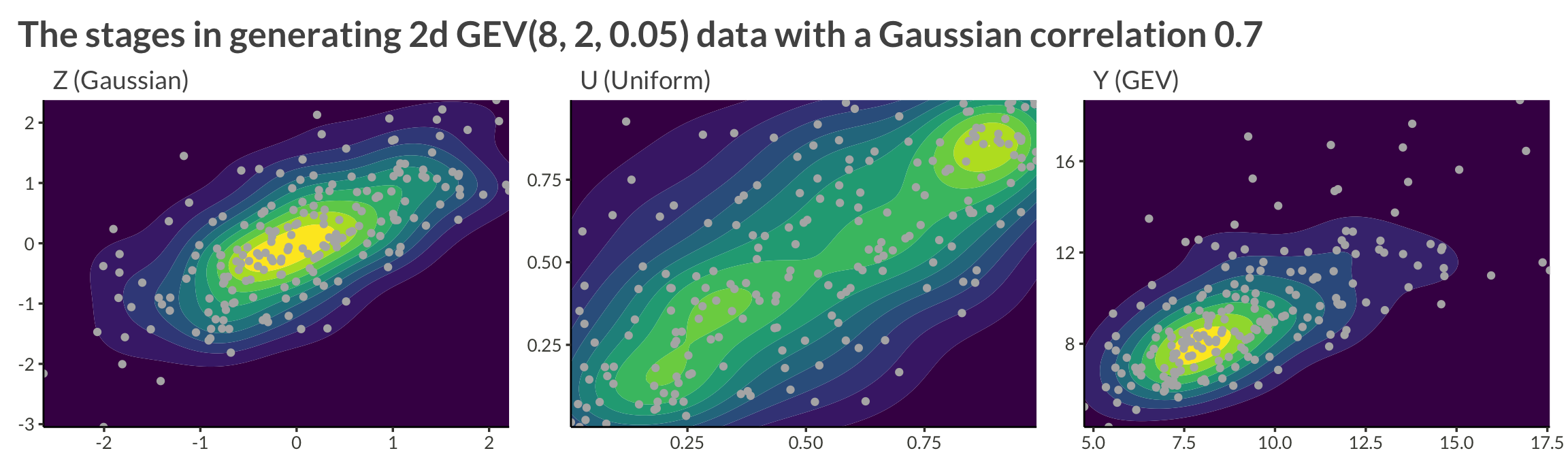
Let’s sample from a two-dimensional process with GEV(8, 2, 0.05) margins and a Gaussian copula with correlation \(\rho = 0.7\).
R <- matrix(c(1, 0.7, 0.7, 1), nrow = 2)
set.seed(1)
X <- mvtnorm::rmvnorm(
  n = 200,
  sigma = R
)

X |>
  as_tibble() |>
  mutate(
    id = row_number()
  ) |>
  pivot_longer(c(-id), names_to = "variable", values_to = "Z") |>
  mutate(
    U = pnorm(Z),
    Y = evd::qgev(U, loc = 8, scale = 2, shape = 0.05)
  ) |>
  pivot_longer(c(-id, -variable)) |>
  pivot_wider(names_from = variable, values_from = value) |>
  mutate(
    name = fct_relevel(name, "Z", "U", "Y") |>
      fct_recode(
        "Z (Gaussian)" = "Z",
        "U (Uniform)" = "U",
        "Y (GEV)" = "Y"
      )
  ) |>
  group_by(name2 = name) |>
  group_map(
    function(data, ...) {
      data |>
        ggplot(aes(V1, V2)) +
        geom_density_2d_filled() +
        geom_point(col = "grey70") +
        coord_cartesian(expand = FALSE) +
        theme(legend.position = "none") +
        labs(
          x = NULL,
          y = NULL,
          subtitle = data$name
        )
    }
  ) |>
  wrap_plots() +
  plot_annotation(
    title = "The stages in generating 2d GEV(8, 2, 0.05) data with a Gaussian correlation 0.7"
  )
R scripts used for simulating the data
The simulated data have GEV margins and an AR(1) Gaussian copula. The steps in simulating the data are as follows.
First, a correlation matrix is generated that encodes an AR(1) process with correlation \(\rho\). To create this correlation matrix, we specify the precision matrix, \(Q\), via
\[ Q = \frac{1}{1 - \rho^2}\begin{bmatrix} 1 & -\rho & \dots & \dots & \vdots\\ -\rho & 1 + \rho^2 & -\rho & \ddots & \vdots \\ \vdots & \ddots & \ddots & \ddots & \vdots \\ \vdots & \ddots &-\rho & 1 + \rho^2 & -\rho \\ \vdots & \dots & \dots & -\rho & 1 \end{bmatrix}. \]
This gives us the correlation matrix, R, where
\[ R = Q^{-1} = \begin{bmatrix} 1 & \rho & \rho^2 & \dots & \rho^n\\ \rho & 1 & \rho & \ddots & \rho^{n-1} \\ \vdots & \ddots & \ddots & \ddots & \vdots \\ \rho^{n-1} & \ddots &\rho & 1 & \rho \\ \rho^n & \dots & \dots & \rho & 1 \end{bmatrix}. \]
make_AR_cor_matrix_1d <- function(n_id, rho = 0.5) {
  P <- matrix(
    0,
    nrow = n_id,
    ncol = n_id
  )
  diag(P) <- 1
  for (i in seq(1, n_id - 1)) {
    P[i, i + 1] <- -rho
  }

  for (i in seq(2, n_id)) {
    P[i, i - 1] <- -rho
  }

  for (i in seq(2, n_id - 1)) {
    P[i, i] <- 1 + rho^2
  }

  P <- P / (1 - rho^2)

  P_cor <- solve(P)
  P_cor
}

n_id <- 5
rho <- 0.5

R <- make_AR_cor_matrix_1d(n_id = n_id, rho = rho)
R
[,1] [,2] [,3] [,4] [,5]
[1,] 1.0000 0.500 0.25 0.125 0.0625
[2,] 0.5000 1.000 0.50 0.250 0.1250
[3,] 0.2500 0.500 1.00 0.500 0.2500
[4,] 0.1250 0.250 0.50 1.000 0.5000
[5,] 0.0625 0.125 0.25 0.500 1.0000We then use the well-known fact that if
\[ \mathbf X \sim \mathrm{MVNorm}\left(\boldsymbol \mu, \Sigma\right), \]
then
\[ \boldsymbol X = \boldsymbol \mu + L \boldsymbol Z, \]
where \(\boldsymbol Z \sim \mathrm{Normal}(\boldsymbol 0, I)\) and \(L\) is the Cholesky decomposition of \(R\), or \(LL^T = \Sigma\).
In our case, we want \(\mathbf X\) to have mean 0 and covariance matrix \(R\), so we write
\[ \mathbf X = L\mathbf Z \]
where \(LL^T = R\).
We can skip the manual Cholesky factorization and simply use the {mvtnorm} package.
sample_gaussian_variables <- function(cor_matrix, n_replicates) {
  mvtnorm::rmvnorm(
    n = n_replicates,
    sigma = cor_matrix
  )
}

R |>
  sample_gaussian_variables(n_replicates = 1)
[,1] [,2] [,3] [,4] [,5]
[1,] 1.427875 1.837133 -0.1348893 -0.3970323 -0.4613493We will want more than one observation from each “site”, so we write a helped function for tidying this output into a tibble.
tidy_mvgauss <- function(mvnorm_matrix) {
  colnames(mvnorm_matrix) <- seq_len(ncol(mvnorm_matrix))

  mvnorm_matrix |>
    dplyr::as_tibble() |>
    dplyr::mutate(
      replicate = dplyr::row_number(),
      .before = `1`
    ) |>
    tidyr::pivot_longer(
      c(-replicate),
      names_to = "id", names_transform = as.numeric,
      values_to = "Z"
    )

}

n_replicates <- 10
mvnorm_data <- R |>
  sample_gaussian_variables(n_replicates = n_replicates) |>
  tidy_mvgauss()

mvnorm_data |>
  filter(replicate <= 5) |>
  pivot_wider(names_from = replicate, values_from = Z) |>
  gt() |>
  tab_spanner(
    columns = -id,
    label = "Replicate"
)| id | Replicate | ||||
|---|---|---|---|---|---|
| 1 | 2 | 3 | 4 | 5 | |
| 1 | -0.4364007 | -0.1443106 | 0.7080631 | 1.1388723 | 1.0330390 |
| 2 | -0.4017539 | 0.6923541 | 0.9544816 | -0.4595604 | -1.3986486 |
| 3 | -0.1161437 | 0.9328314 | -0.1228664 | -0.4689164 | -1.1884398 |
| 4 | 1.0500406 | -0.5297770 | -0.8530328 | -1.5227378 | -1.0434809 |
| 5 | -0.3607882 | -0.5568922 | 1.3144552 | 0.1006016 | -0.9255078 |
Now our data, \(\mathbf X\), is multivariate normal with dependence structure according to an AR(1) process, but marginally each \(X_1\) is standard normal. To transform this data to a GEV dataset, we simply use the standard normal CDF on each \(X_i\) to transform it to \([0, 1]\), then we use the GEV quantile function to transform that to a GEV distributed variable.
mvnorm_to_gev <- function(mvnorm_data, gev_params) {

  mvnorm_data |>
    dplyr::mutate(
      U = pnorm(Z)
    ) |>
    dplyr::inner_join(
      gev_params,
      by = dplyr::join_by(id)
    ) |>
    dplyr::mutate(
      y = purrr:::pmap_dbl(
        list(U, mu, sigma, xi),
        \(U, mu, sigma, xi) evd::qgev(p = U, loc = mu, scale = sigma, shape = xi)
      )
    )
}

gev_params <- expand_grid(
  mu = 6,
  sigma = 3,
  xi = 0.1,
  id = seq_len(n_id)
)

gev_data <- mvnorm_data |>
  mvnorm_to_gev(gev_params = gev_params)

gev_data |>
  select(-mu, -sigma, -xi) |>
  gt() |>
opt_interactive()Let’s create a function that plots heat maps for each of the three representations of the data
We want the color scales to be free, so we use group_map() and wrap_plots() instead of facet_wrap()
plot_data <- function(data) {
  data |>
    select(replicate, id, Z, U, y) |>
    pivot_longer(c(-replicate, -id)) |>
    mutate(
      name = fct_relevel(name, "Z", "U", "y"),
      name2 = name
    ) |>
    group_by(name) |>
    group_map(
      function(data, ...) {
        data |>
          ggplot(aes(id, replicate, fill = value)) +
          geom_raster() +
          scale_fill_viridis_c() +
          coord_cartesian(expand = FALSE) +
          theme(legend.position = "none") +
          labs(
            subtitle = data$name2
          )
      }
    ) |>
    wrap_plots() +
    plot_layout(nrow = 1) +
    plot_annotation(
      title = "Heatmaps of the three data representations",
      subtitle = "Z: Normal | U: Uniform | y: GEV"
    )
}gev_data |>
plot_data()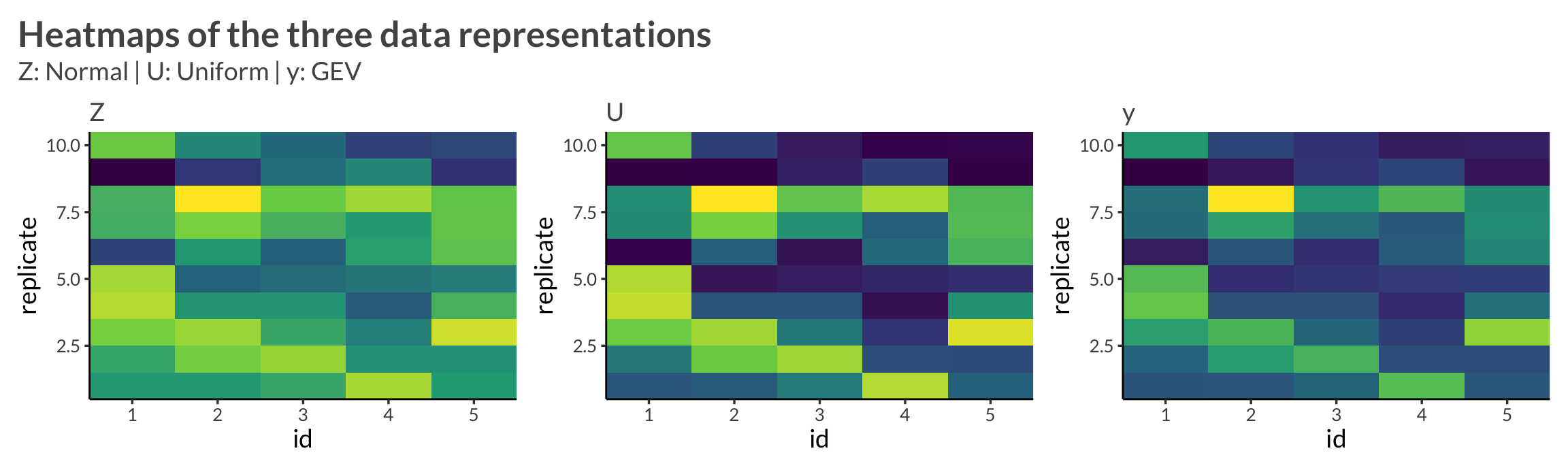
It’s nice to wrap this process in a single function
make_data <- function(gev_params, n_replicate, rho) {

  make_AR_cor_matrix_1d(n_id = nrow(gev_params), rho = rho) |>
    sample_gaussian_variables(n_replicates = n_replicate) |>
    tidy_mvgauss() |>
    dplyr::mutate(
      U = pnorm(Z)
    ) |>
    dplyr::inner_join(
      gev_params,
      by = dplyr::join_by(id)
    ) |>
    dplyr::mutate(
      y = purrr::pmap_dbl(
        list(U, mu, sigma, xi),
        \(U, mu, sigma, xi) evd::qgev(p = U, loc = mu, scale = sigma, shape = xi)
      )
    )
}
Let’s see how the data look if we make it larger and increase the correlation
n_id <- 40
n_replicates <- 100

gev_params <- expand_grid(
  mu = 6,
  sigma = 3,
  xi = 0.1,
  id = seq_len(n_id)
)

d <- make_data(gev_params, n_replicates, rho = 0.95)
We see that with higher neighbor correlations we get obvious horizontal stripes corresponding to a large amount of dependence within each replicate.
d |> plot_data()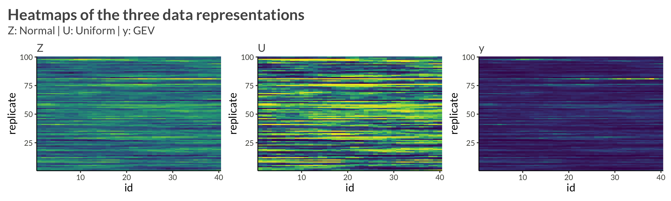
We can fit the AR(1) model directly using Stan.
functions {
  real normal_ar1_lpdf(vector x, real rho) {
    int N = num_elements(x);
    real out;
    real log_det = - (N - 1) * (log(1 + rho) + log(1 - rho)) / 2;
    vector[N] q;
    real scl = sqrt(1 / (1 - rho^2));

    q[1:(N - 1)] = scl * (x[1:(N - 1)] - rho * x[2:N]);
    q[N] = x[N];

    out = log_det - dot_self(q) / 2;

    return out;
  }

  real normal_copula_ar1_lpdf(vector U, real rho) {
    int N = rows(U);
    vector[N] Z = inv_Phi(U);
    return normal_ar1_lpdf(Z | rho) + dot_self(Z) / 2;
  }

  real gev_cdf(real y, real mu, real sigma, real xi) {
    if (abs(xi) < 1e-10) {
      real z = (y - mu) / sigma;
      return exp(-exp(z));
    } else {
      real z = 1 + xi * (y - mu) / sigma;
      if (z > 0) {
        return exp(-pow(z, -1/xi));
      } else {
        reject("Found incompatible GEV parameter values");
      }
    }
  }

  real gev_lpdf(real y, real mu, real sigma, real xi) {
    if (abs(xi) < 1e-10) {
      real z = (y - mu) / sigma;
      return -log(sigma) - z - exp(-z);
    } else {
      real z = 1 + xi * (y - mu) / sigma;
      if (z > 0) {
        return -log(sigma) - (1 + 1/xi) * log(z) - pow(z, -1/xi);
      } else {
        reject("Found incompatible GEV parameter values");
      }
    }
  }
}

data {
  int<lower = 0> n_replicate;
  int<lower = 0> n_id;
  array[n_replicate, n_id] real y;
  array[n_replicate, n_id] real y_test;
}

parameters {
  real<lower = 0> mu;
  real<lower = 0> sigma;
  real<lower = -0.5, upper = 1> xi;
  real<lower = -1, upper = 1> rho;
}

model {
  for (i in 1:n_replicate) {
    vector[n_id] U;
    for (j in 1:n_id) {
      U[j] = gev_cdf(y[i, j] | mu, sigma, xi);
      target += gev_lpdf(y[i, j] | mu, sigma, xi);
    }
    target += normal_copula_ar1_lpdf(U | rho);
  }
}

generated quantities {
  real log_lik = 0;
  {

    for (i in 1:n_replicate) {
      vector[n_id] U;
      for (j in 1:n_id) {
        U[j] = gev_cdf(y_test[i, j] | mu, sigma, xi);
        log_lik += gev_lpdf(y_test[i, j] | mu, sigma, xi);
      }
      log_lik += normal_copula_ar1_lpdf(U | rho);
    }
  }

}functions {
real gev_lpdf(real y, real mu, real sigma, real xi) {
if (abs(xi) < 1e-10) {
real z = (y - mu) / sigma;
return -log(sigma) - z - exp(-z);
} else {
real z = 1 + xi * (y - mu) / sigma;
if (z > 0) {
return -log(sigma) - (1 + 1/xi) * log(z) - pow(z, -1/xi);
} else {
reject("Found incompatible GEV parameter values");
}
}
}
}
data {
int<lower = 0> n_replicate;
int<lower = 0> n_id;
array[n_replicate, n_id] real y;
array[n_replicate, n_id] real y_test;
}
parameters {
real<lower = 0> mu;
real<lower = 0> sigma;
real<lower = -0.5, upper = 1> xi;
}
transformed parameters {
}
model {
for (i in 1:n_replicate) {
for (j in 1:n_id) {
target += gev_lpdf(y[i, j] | mu, sigma, xi);
}
}
}
generated quantities {
real log_lik = 0;
{
for (i in 1:n_replicate) {
for (j in 1:n_id) {
log_lik += gev_lpdf(y_test[i, j] | mu, sigma, xi);
}
}
}
}We can’t fit this model directly using one stan file. What we do is:
functions {
  real gev_cdf(real y, real mu, real sigma, real xi) {
    if (abs(xi) < 1e-10) {
      real z = (y - mu) / sigma;
      return exp(-exp(z));
    } else {
      real z = 1 + xi * (y - mu) / sigma;
      if (z > 0) {
        return exp(-pow(z, -1/xi));
      } else {
        reject("Found incompatible GEV parameter values");
      }
    }
  }

  real gev_lpdf(real y, real mu, real sigma, real xi) {
    if (abs(xi) < 1e-10) {
      real z = (y - mu) / sigma;
      return -log(sigma) - z - exp(-z);
    } else {
      real z = 1 + xi * (y - mu) / sigma;
      if (z > 0) {
        return -log(sigma) - (1 + 1/xi) * log(z) - pow(z, -1/xi);
      } else {
        reject("Found incompatible GEV parameter values");
      }
    }
  }

  real normal_prec_chol_lpdf(vector x, array[] int n_values, array[] int index, vector values, real log_det) {
    int N = num_elements(x);
    int counter = 1;
    vector[N] q = rep_vector(0, N);

    for (i in 1:N) {
      for (j in 1:n_values[i]) {
        q[i] += values[counter] * x[index[counter]];
        counter += 1;
      }
    }

    return log_det - dot_self(q) / 2;

  }

  real normal_copula_prec_chol_lpdf(vector U, array[] int n_values, array[] int index, vector value, real log_det) {
    int N = rows(U);
    vector[N] Z = inv_Phi(U);

    return normal_prec_chol_lpdf(Z | n_values, index, value, log_det) + dot_self(Z) / 2;
  }

}

data {
  int<lower = 0> n_replicate;
  int<lower = 0> n_id;
  array[n_replicate, n_id] real y;
  array[n_replicate, n_id] real y_test;

  int<lower = 0> n_nonzero_chol_Q;
  real log_det_Q;
  array[n_id] int n_values;
  array[n_nonzero_chol_Q] int index;
  vector[n_nonzero_chol_Q] value;
}

parameters {
  real<lower = 0> mu;
  real<lower = 0> sigma;
  real<lower = -0.5, upper = 1> xi;
}

model {
  for (i in 1:n_replicate) {
    for (j in 1:n_id) {
      target += gev_lpdf(y[i, j] | mu, sigma, xi);
    }
  }
}

generated quantities {
  real log_lik = 0;
  {

    for (i in 1:n_replicate) {
      vector[n_id] U;
      for (j in 1:n_id) {
        U[j] = gev_cdf(y_test[i, j] | mu, sigma, xi);
        log_lik += gev_lpdf(y_test[i, j] | mu, sigma, xi);
      }
      log_lik += normal_copula_prec_chol_lpdf(U | n_values, index, value, log_det_Q);
    }
  }

}